Analyzing a single damped sinusoid
This is the simplest possible example: we analyze a single damped sinusoid in white Gaussian noise. We use this case study to demonstrate some basic features of ringdown, including:
how to measure generic frequencies and damping rates
how to set up a fit and run it
how to make some useful plots
Let’s get started!
[1]:
%matplotlib inline
%config InlineBackend.figure_format = 'retina'
[2]:
# disable numpy multithreading to avoid conflicts
# with jax multiprocessing in numpyro
import os
os.environ["OMP_NUM_THREADS"] = "1"
import numpy as np

# import numpyro and set it up to use 4 CPU devices
import numpyro
numpyro.set_host_device_count(4)

# disable some warning shown by importing LALSuite from a notebook
import warnings
warnings.filterwarnings("ignore", "Wswiglal-redir-stdio")

import matplotlib.pyplot as plt
import arviz as az
import seaborn as sns
import pandas as pd
import ringdown as rd

sns.set_theme(context='notebook', palette='colorblind')
Data
Let’s create the simplest possible signal and add Gaussian noise to it. Although ringdown contains tools to create and maniuplate more complex ringdown and inspiral-merger-ringdown waveforms, we do not need that for this very simple example.
Signal
First, create a time array based on a specified sampling rate and duration; center it around a target time \(t_0\).
[3]:
# define sampling rate and duration (make these powers of two)
fsamp = 8192
duration = 4
t0 = 0

delta_t = 1/fsamp
tlen = int(round(duration / delta_t))
epoch = t0 - 0.5*tlen*delta_t

time = np.arange(tlen)*delta_t + epoch
We can now use the above timestmps to create a simulated damped sinusoid starting at \(t_0\); for good measure, let’s extend the signal before \(t_0\) to be a corresponding ring-up (the inference is insensitive to what happens before \(t_0\), so we can always just let the signal vanish for \(t < t_0\), as long as no step in the data conditioning involves taking a Fourier transform—which is true in the example here).
[4]:
wf_kws = dict(
    A = 5,
    phi = 0,
    f = 250,
    gamma = 250,
)

def get_signal(time, A, phi, f, gamma):
    s = A*np.cos(2*np.pi*f*(time-t0) - phi)*np.exp(-gamma*abs(time-t0))
    return rd.Data(s, index=time)

signal = get_signal(time, **wf_kws)
[5]:
signal.plot(label='signal')
plt.axvline(t0, ls=':', c='k', label='start time')
plt.xlim(-0.03, 0.03)
plt.xlabel('time (s)')
plt.ylabel('strain')
plt.legend();

Noise
Let’s add some white Gaussian noise to the signal to obtain our data. This means the autocorrelation function (ACF) of the noise will be \(\rho(\tau) = \delta(\tau)\).
[6]:
rng = np.random.default_rng(12345)
data = signal + rng.normal(0, 1, len(signal))
[7]:
data.plot(label='data')
signal.plot(label='signal')
plt.axvline(t0, ls=':', c='k', label='start time')
plt.xlim(-0.03, 0.03)
plt.xlabel('time (s)')
plt.ylabel('strain')
plt.legend();

For our ringdown analysis, we will need the ACFs corresponding to the noise, which we could estimate empirically from the data; in this case, however, we know the ACF to be a delta function at the origin (corresponding to standard Gaussian noise).
[8]:
acf = rd.AutoCovariance(np.zeros_like(data), delta_t=data.delta_t)
acf.iloc[0] = 1
Of course, when working with white noise it is unnecessary to work with the ACF: all we have is a variance (in this case, \(\sigma^2 = 1\)) and the likelihood simplifies drastically. However, in real life we never have white noise, so ringdown expects an ACF and cannot currently accomodate a scalar variance.
Fit
We are now ready to analyze the ringdown! Let’s create a Fit object and set up the analysis. To do this, we first need to specify the model to be fit and the number (or kind) of modes to be used. In this case, we will be using the ftau model, which is parameterized in terms of damped sinusoids with generic frequencies \(f_n\), damping rates \(\gamma_n = 1/\tau_n\), amplitudes \(A_n\), and phases \(\phi_n\), defined such that successive modes are ordered in terms of
damping rate (\(\gamma_n < \gamma_{n+1}\)); for this is example, we will only inject and recover a single mode. Since we are simulating a simple damped sinusoid in a single data stream, we need to use the single_polarization argument so that the fit does not look for two gravitational wave polarizations.
[9]:
fit = rd.Fit(modes=1, single_polarization=True)
Since we already have the data and ACFs, we can add those directly to the fit now.
[10]:
fit.add_data(data, acf=acf)
Now, let’s specify a target for the analysis, i.e., the desired start time and analysis segment duration.
Note
We will pick a very short duration to make this is example run fast, but in a real analysis this should be set based on the timescale imposed by the whitening filter and might well exceed the duration of the unwhitened signal.
[11]:
fit.set_target(t0, duration=0.03)
Finally, let’s set some reasonable prior based on our knowledge of the true signal.
[12]:
fit.update_model(a_scale_max=20, f_min=50, f_max=500, g_min=50, g_max=500)
fit.model_settings
[12]:
{'single_polarization': True,
 'a_scale_max': 20,
 'f_min': 50,
 'f_max': 500,
 'g_min': 50,
 'g_max': 500}
Our fit is ready to go; run it! This should take around 15 s or less in a modern laptop.
[13]:
fit.run()
WARNING:root:running with float32 precision
Result
After the run is done, fit.result contains an Arviz object giving our results:
[14]:
az.summary(fit.result, var_names=['a', 'phi', 'f', 'g'])
[14]:
| mean | sd | hdi_3% | hdi_97% | mcse_mean | mcse_sd | ess_bulk | ess_tail | r_hat | |
|---|---|---|---|---|---|---|---|---|---|
| a[0] | 5.228 | 0.446 | 4.307 | 5.988 | 0.008 | 0.006 | 3165.0 | 2796.0 | 1.0 |
| phi[0] | -0.075 | 0.106 | -0.271 | 0.126 | 0.002 | 0.001 | 3612.0 | 3321.0 | 1.0 |
| f[0] | 246.559 | 5.550 | 236.237 | 256.957 | 0.092 | 0.065 | 3682.0 | 2463.0 | 1.0 |
| g[0] | 226.108 | 26.744 | 178.042 | 277.127 | 0.505 | 0.366 | 2892.0 | 2143.0 | 1.0 |
We can plot a trace, and see visually that the sampling seems OK for all the different chains (chains are represented by a different linestyle):
[15]:
az.plot_trace(fit.result, var_names=['a', 'phi', 'f', 'g']);
plt.subplots_adjust(hspace=0.5)

This is a very useful plot to diagnose the quality of a fit.
Posterior
We can also make a corner plot using Seaborn, and check that the posterior supports the truth.
[16]:
df = pd.DataFrame({
    r'$A$': fit.result.posterior.a.values.flatten(),
    r'$\phi$': fit.result.posterior.phi.values.flatten(),
    r'$f / \mathrm{Hz}$': fit.result.posterior.f.values.flatten(),
    r'$\gamma  / \mathrm{Hz}$': fit.result.posterior.g.values.flatten()
})
pg = sns.PairGrid(df, diag_sharey=False, corner=True)
pg.map_diag(sns.kdeplot);
pg.map_lower(sns.scatterplot, marker='.', alpha=0.02);
pg.map_lower(rd.utils.kdeplot, levels=[0.9, 0.5, 0.1]);

# plot true values
for i, vi in enumerate(wf_kws.values()):
    for j, vj in enumerate(wf_kws.values()):
        if i >= j:
            pg.axes[i,j].axvline(vj, ls=':')
            if i != j:
                pg.axes[i,j].axhline(vi, ls=':')

Reconstructions
Get mean signal reconstructions at each detector and plot them against the truth.
[17]:
# median reconstruction and 90%-credible envelope
wfs = [np.quantile(fit.result.h_det.values, q, axis=(0,1))[0,:]
       for q in [0.5, 0.95, 0.05]]
wfs = [rd.Data(wf, index=fit.analysis_data[None].time) for wf in wfs]
[18]:
# plot reconstructions computed above
m, u, d = wfs
l, = plt.plot(m, label='measured')
plt.fill_between(m.time, u, d, color=l.get_color(), alpha=0.25)

# plot truth (using time mask to select right times)
plt.plot(signal[m.time], c='k', ls='--', label='truth')

plt.xlabel('time (s)')
plt.ylabel('strain')
plt.legend();

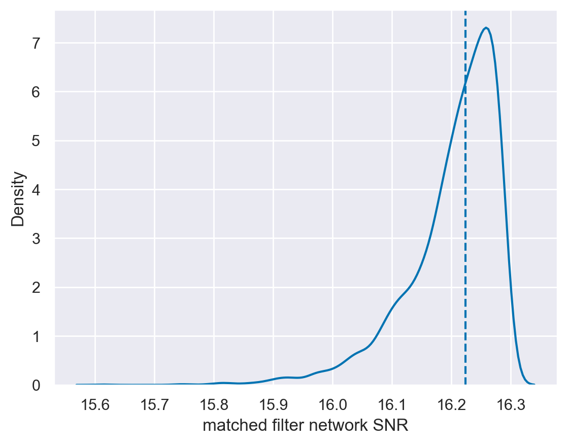
Let’s compute the recovered matched filter SNR, defined as \(\rho = \left\langle h \mid d \right\rangle / \left\langle h \mid h \right\rangle\). We can obtain a posterior on the recovered matched filter SNR by computing this quantity from random draws of the posterior; the Fit object can do this automatically (and efficiently) for us.
[19]:
snrs_mf = fit.result.compute_posterior_snrs(optimal=False, network=True)
Also compute the injected matched-filter SNR for reference:
[20]:
injsnr_mf = np.dot(signal[m.time], data[m.time]) / np.linalg.norm(signal[m.time])
[21]:
sns.kdeplot(snrs_mf)
plt.axvline(injsnr_mf, ls='--');
plt.xlabel('matched filter network SNR');
Saving
If you want, you can save the fit result to disk as follows:
[22]:
fit.result.to_netcdf('myfit.nc')
[22]:
'myfit.nc'
And you can load that by doing:
[23]:
cached_result = rd.Result.from_netcdf('myfit.nc')
This new object, cached_result, will be the same as the original fit.result.
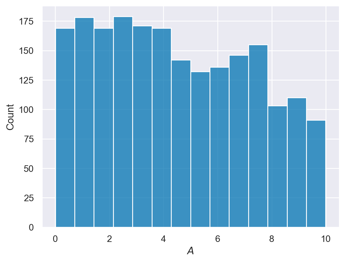
Bonus: What’s the prior?
The above posterior was obtained under ringdowns default prior given the provided settings. This prior is designed to be flat in amplitude below a_scale_max/2, and tapering smoothly for higher values. You can always check the prior explicitly by rerunning your Fit using the prior=True option; the result will be saved in fit.prior.
[24]:
fit.run(prior=True)
WARNING:root:running with float32 precision
[25]:
az.plot_trace(fit.prior, var_names=['a', 'phi', 'f', 'g']);

[26]:
a = fit.prior.posterior.a.values.flatten()
sns.histplot(a[a<fit.model_settings['a_scale_max']/2], label='posterior');
plt.xlabel('$A$');
Note
This page was generated from a Jupyter notebook that can be downloaded here.